Trend Line Example: How to Read Changes Over Time

You've been logging your mood, but the chart still looks like a string of good days and difficult days. Say you've recorded a score on a 1-to-10 scale every day for six weeks. You want to know whether things are moving in a direction, not just whether today felt better than yesterday.
A trend line helps answer that narrower question. This worked trend line example shows how to calculate it, check the arithmetic, and describe the result without turning a personal observation into a claim about what caused it.
Table of Contents
- What a Trend Line Shows in Plain Terms
- Fitting a Line to Mood Scores
- Reading the Slope Without Overreading It
- Checking Whether the Trend Is Real
- Smoothing Data So the Trend Stands Out
- Turn Your Own Data Into a Trend Line
What a Trend Line Shows in Plain Terms
A trend line is a mathematical summary of the overall direction through a set of observations. Think of a rough walking path across a hill: the path dips and rises, while a straight route across the hillside summarizes whether you're generally climbing or descending.
Your daily mood scores are the rough path. The line summarizes their direction, but it doesn't replace the individual experiences.
The standard straight-line model is ŷ = a + bt, where t represents time, a is the intercept, and b is the slope, as explained in Duke University's guide to linear trend models. The hat over y means fitted value, the model's estimate rather than the score you logged.
Read the equation as a sentence
Each part has a practical meaning:
- Time, t: The position of an observation along the horizontal axis.
- Intercept, a: The fitted level when time equals zero. It isn't necessarily your actual first score.
- Slope, b: The average change in fitted mood for each additional time step.
Keep the time unit explicit. A slope measured per day means something different from one measured per weekly entry. If you skip entries, calendar time and observation number no longer mean the same thing.
The visual distinction is simple: the points show individual observations, while the line shows their fitted direction.

Why the line doesn't just join the endpoints
Ordinary least squares fits the line using all the observations. It chooses the intercept and slope that minimize the sum of squared vertical gaps between the observed points and the line.
Squaring prevents positive and negative gaps from canceling, and gives larger gaps more influence. That's why a fitted line can look different from a line drawn between the first and last scores.
Reading rule: A positive slope indicates an upward trend, a negative slope indicates a downward trend, and a slope near zero indicates little systematic movement.
Fitting a Line to Mood Scores
Use Excel or Google Sheets to make the calculation checkable:
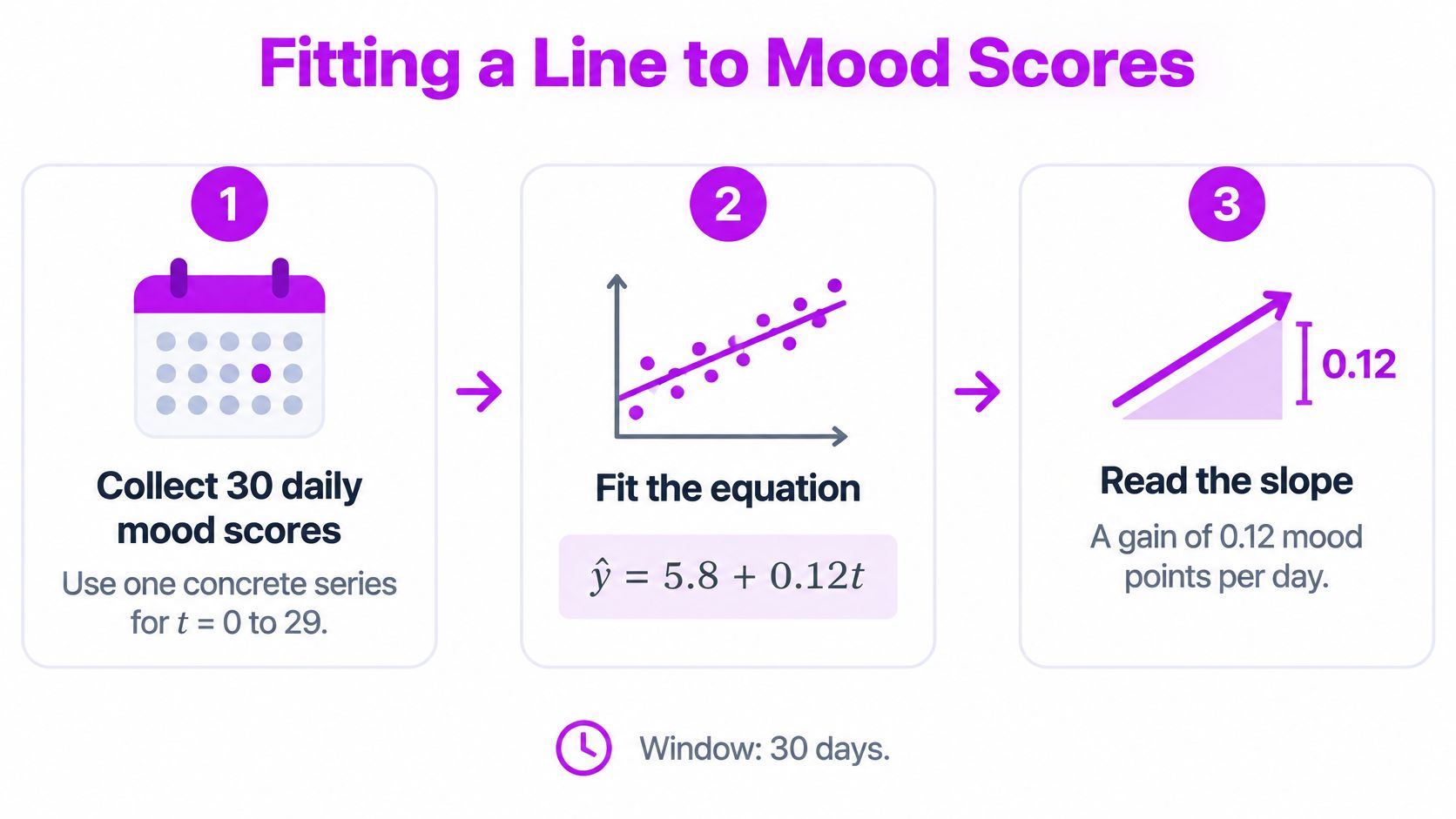
- Set up the columns. Put day numbers in column A and mood scores in column B, with headers above the entries. For this hypothetical example, use 30 daily observations, indexed from t = 0 to 29.
- Calculate the slope. Enter
=SLOPE(B2:B31,A2:A31)in a separate cell. This returns b. - Calculate the intercept. Enter
=INTERCEPT(B2:B31,A2:A31)in another cell. This returns a. - Create a scatter chart. Select the day and mood columns, insert a scatter chart, and add a linear trendline. Display its equation.
- Compare the results. The chart equation should match the slope and intercept cells, allowing for display rounding. Show more decimal places if they appear inconsistent.
Before collecting real entries, choose consistent descriptions for your scores. A daily mood rating scale helps you avoid changing what a rating means halfway through the tracking period.
Build a series you can reproduce
For a fully checkable teaching example, generate synthetic scores rather than pretending an equation came from undisclosed observations.
Enter the day numbers in A2:A31. In B2, enter =5.8+0.12*A2+CHOOSE(MOD(A2,3)+1,0.2,-0.4,0.2) and fill down to B31. This hypothetical series adds a repeating pattern of small deviations to the example line ŷ = 5.8 + 0.12t.
The deviations balance both in total and in their relationship with time. Consequently, the spreadsheet returns a slope of 0.12 and an intercept of 5.8, apart from possible floating-point rounding. These are demonstration scores, not evidence about anyone's mood or microdosing outcomes.
The process can be summarized visually:
Fitted mood values from the example equation
| Observation number (t) | Fitted mood (5.8 + 0.12t) |
|---|---|
| 0 | 5.8 |
| 5 | 6.4 |
| 10 | 7.0 |
| 20 | 8.2 |
| 29 | 9.28, or 9.3 rounded |
For example, the hypothetical fitted value at t = 5 is 5.8 + 0.12 × 5 = 6.4. Every table entry stays within the observed time range; extending the calculation beyond the last observation would be extrapolation.
Compare a point with the line
The table reads the fitted line, not the raw scores. In the synthetic series, the score at t = 5 is 6.6, while its fitted value is 6.4, giving a residual of +0.2, calculated as observed minus fitted.
That gap doesn't invalidate the upward direction. Least squares accommodates deviations across the whole series rather than requiring every point to touch the line.
Reading the Slope Without Overreading It
The most common mistake is treating an upward line as proof that an intervention worked. A slope describes how the recorded outcome changed with time, not why it changed.
In the hypothetical mood example, the fitted increase is 0.12 points per observation. That rate could coexist with changes in sleep, work pressure, expectations, relationships, or logging habits. The equation doesn't separate those explanations.
This distinction matters especially for microdosing journals. A longitudinal observational study published in Scientific Reports followed 953 psilocybin microdosers and 180 non-microdosing comparators for approximately 30 days and reported observed improvements in mood and mental health among microdosers. Because the study was observational, those changes don't establish that microdosing caused them.
Replace the causal claim
For the hypothetical series, write:
Mood increased at an estimated rate of 0.12 points per observation during this window.
Don't substitute a claim that the intervention improved mood. That adds a causal conclusion the fitted line cannot supply.
Other interpretation errors are easier to catch once you know where to look:
- Endpoint selection: Joining only the first and last points ignores everything recorded between them.
- Long-range projection: Extending a straight line far beyond the observed days assumes the same rate continues. A bounded mood scale makes that assumption especially fragile.
- Single-day reactions: An unusually high or low entry deserves context, not an immediate declaration of a new trend.
- Unequal comparisons: Slopes from different calendar windows or different logging densities aren't interchangeable. Match the time unit and inspect coverage before comparing them.
Keep dose-day experiences separate from the broader question of sustained change. A short-lived difference around an entry and a gradual shift across a tracking period are different patterns, even when they appear on the same chart.
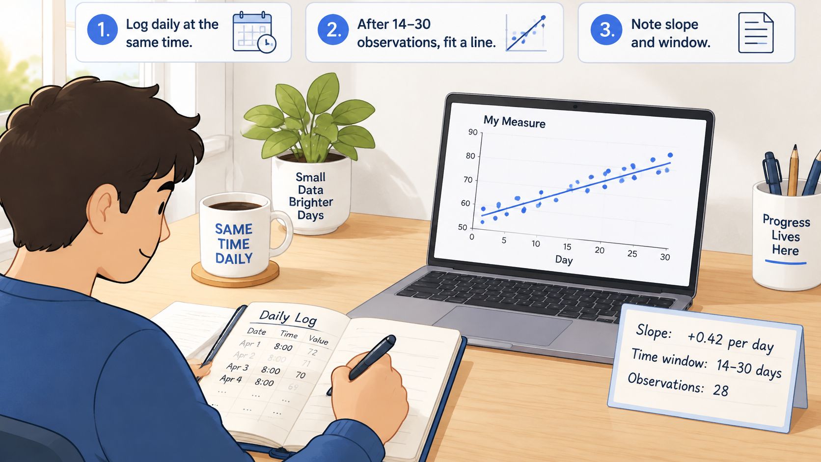
Before sharing a result, state the slope, the time window, and the number of observations together. Those details tell the reader what was summarized.
Checking Whether the Trend Is Real
A positive estimate can look convincing even when it's too uncertain to distinguish from a flat trend. Here, real means supported as a linear association under the model's assumptions, not proven beneficial or causal.
Consider a separate worked example: ŷ = 6.2 + 0.04t, with an estimated increase of 0.04 mood points per day, equivalent to approximately 0.28 points per week. Using the slope-confidence-interval method described in Penn State's regression inference guidance, a standard error of 0.015 across 30 observations gives an approximate 95% interval of 0.009 to 0.071 points per day.
Work through the uncertainty
For that hypothetical calculation, the interval is slope ± t multiplier × standard error. With 28 degrees of freedom, the multiplier is about 2.05, so the arithmetic is 0.04 ± 2.05 × 0.015, or approximately 0.04 ± 0.031.
Because the interval excludes zero, it supports a positive linear association during the recorded period. It doesn't establish that microdosing caused the change; the distinction between correlation and causation still applies.
A confidence interval measures uncertainty within a model. It doesn't rescue a model that poorly represents the observations.
Run the remaining checks in order
- Count valid entries. Choose a minimum before interpreting results. For example, you might use 14 logged days as a provisional review threshold, not a clinically validated cutoff or a guarantee of reliability.
- Inspect residuals. Plot observed minus fitted scores against time. Curvature suggests the straight line misses a changing pattern; isolated large gaps flag unusual observations; a widening spread suggests changing variability.
- Check missing entries. Leave unlogged days blank, not zero. Use elapsed calendar days so gaps retain their true position in time.
Also display R-squared, the share of observed variation explained by the fitted line. A statistically clear slope can still explain little of the daily variation, so statistical clarity and a strong descriptive fit aren't the same thing.
Daily scores may also be related to neighboring days. If residuals show that dependence, a basic regression interval may overstate precision.
Be cautious when early gains plateau, logging becomes more frequent during hard weeks, or protocol changes coincide with calendar time. Each situation can make a simple linear summary misleading.
Smoothing Data So the Trend Stands Out
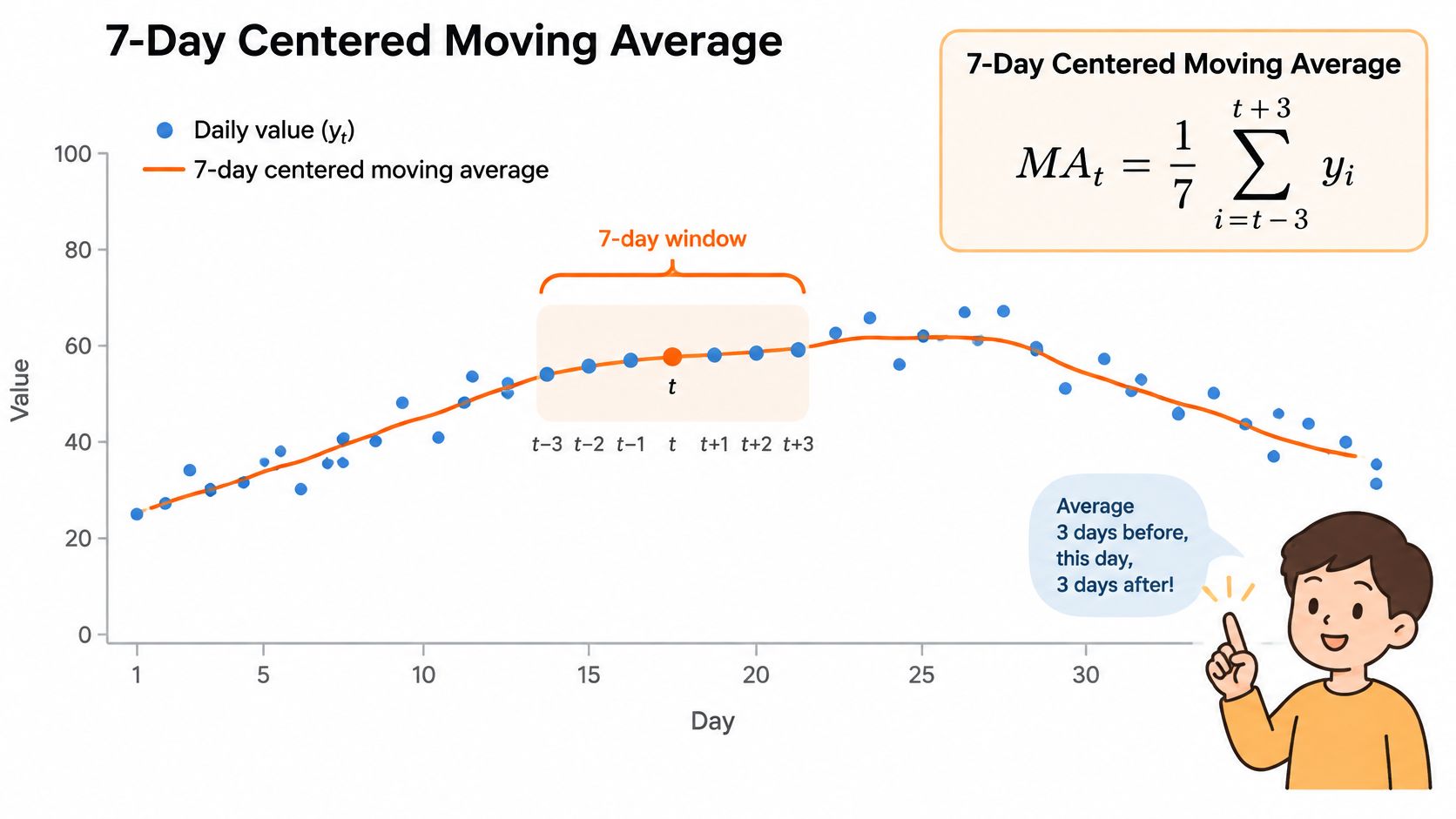
A 7-day centered moving average is the mean of the current day, the three preceding days, and the three following days: MAₜ = (1/7)Σᵢ₌₋₃³ yₜ₊ᵢ, a worked application of the centered-moving-average approach described in CDC time-series methodology.
Unlike regression, this method recalculates a local average as the window moves. It can show bends that a single straight line compresses into one overall direction.
The formula corresponds to a window centered on each plotted day:
Choose the window deliberately
At the edges of this example, within three days of the start or end, average only the available observations and mark the smaller sample. A centered average also needs future entries, so the most recent value remains provisional until the following days are logged.
For a simple window centered exactly on an observed day, use an odd length. The even-length options below use a trailing average of the most recent days instead.
How moving-average window length changes the trend
| Window | Reaction speed | Visible noise | Best use |
|---|---|---|---|
| 3 days (centered) | Fast | High | Spotting a sudden shift around a single dose day |
| 7 days (centered) | Moderate | Moderate | Weekly routines and a sensible starting point |
| 14 days (trailing) | Slow | Low | Two-week protocol cycles |
| 30 days (trailing) | Very slow | Very low | Month-level direction over several cycles |
These are illustrative chart-design choices, not clinical standards. A longer window suppresses more short-term variation but can blur turning points; a shorter window responds faster while retaining more noise. A weekly window also aligns more closely with recurring weekly routines than a month-long average.
For a visual companion to the calculation:
Keep the underlying observations visible
Use these display choices for useful progress visualization:
- Retain raw points: Show daily scores faintly behind the smoothed line.
- Label the method: State the window length and whether it's centered or trailing.
- Mark relevant events: Add dose-day, pause, and schedule-change markers directly to the chart.
- Preserve missingness: Exclude unlogged entries rather than manufacturing low scores.
When comparing periods, use equal calendar windows and report the number of valid observations beside each average. Otherwise, a change in reporting consistency can resemble a change in mood.
Turn Your Own Data Into a Trend Line
Start with a question you can answer descriptively: whether your recorded mood is rising, falling, or staying broadly level during a defined period. You don't need a forecast or a verdict on your whole practice.
Use a routine that keeps collection, calculation, and interpretation separate:
- Log consistently. Record the same measure once a day at roughly the same time. Add brief context when sleep, stress, or your routine changes.
- Schedule a review. As a practical starting routine, review after 14 to 30 observations. Fit the line and record its slope, calendar window, and valid observation count.
- Build a readable chart. Include raw points and, for this workflow, a 7-day centered moving average, clearly labeling provisional edge values.
- Check before concluding. Inspect the confidence interval, residuals, missing entries, and fit rather than relying on the line's angle.
- Write a bounded result. For the uncertainty example, the conclusion is: mood increased at an estimated 0.04 points per day during this 30-day window.
Keep the chart alongside your notes:
Our MicroTrack Insights show mood trends across weeks and months, alongside frequency and time-of-day distributions and pattern detection in your own entries. That gives you a way to review patterns without building every visualization by hand.
Decision rule: If the interval is wide, keep recording for another cycle. If the slope is clear and the entries are complete, change only one tracking or routine variable at a time, without treating the chart as medical advice.
MicroTrack offers structured mood journaling and visual insights for reviewing changes across weeks and months. Visit MicroTrack to start recording consistent entries and give your next trend line a clearer, more interpretable foundation.